![]()
performances, instructions, examples
SuperCalculator is implemented in Javascript, so you can use it only if your browser allows Javascript.
SuperCalculator produces graphs and tables in pop-up windows, so you can fully exploit its resources only if your browser allows pop-ups.
SuperCalculator is intended for educational, non-professional use only; we do not take responsibility for any inaccuracies or errors.
SuperCalculator, unlike an ordinary calculator,
Calculations on integer and rational numbers, represented by fractions or by repeating decimals, are always exact.
Calculations on integer numbers exploit a library of L. Baird.
Rational numbers can be input as fractions or repeating decimals.
In this case the repeated digits must be written between square brackets
([...]). Example: 1.2[34].
The decimal separator in real and rational numbers is the period; commas are not allowed: commas act only as separators between the items of a list.
Real numbers can be input in exponential notation. Example: 1.234e-5.
The letter e must be written lowercase, since the letter 'E', written in capital letters, represents the basis of the natural logarithms.
When calculations generate real numbers, results will be approximated to
the number of digit written in the decimals field (by default 6).
If this number is too high, the computing time may become intolerable.
In the field time you can set the maximum waiting time (in seconds, by default 1).
Numbers in sexagesimal format, used for angular measurements, are expressed by three groups of digits separated by the symbols °, ', " for degrees, primes and seconds. Possible expressions of degrees, primes and seconds in input can be rational numbers; in output these expressions are normalized so that the degrees are expressed by natural numbers, the primes by natural numbers <60 and the seconds by rational numbers < 60.
Example: 12°15'18"+34°56'55.34571"; Sin[30°]; a=15.45°; b=12.18°78'; a+b
The imaginary unit is written as
I. The letter I must be written in capital letters.
Examples:
2I; 1+3I; 5-12I;1/2I; 1/2+3/4I; 1.2[3]I; 1.2-3.4[56]I;Boolean values are represented with the characters T and F, mandatory uppercase.
Using the appropriate operators described below you can perform Boolean calculations.
Examples:
(T&&F)==FT->F;It is possible to make some calculations on matrices and on vectors. Vectors can be written as lists and the matrices as lists of lists.
Example: Det[{{1,2,3},{0,1/2,-3},{a,b,0}}].
The constants selector allows you to enter directly into the input field the values of the most
common mathematical and physical constants.
Other constants can be stored in memory for further usage.
The operators selector allows you to enter directly into the input field the names of the most
common mathematical functions and operators.
To obtain documentation on available operators, use the question mark ? followed by the name of the operator. The uppercase or lowercase format of the characters is irrelevant.
Example: ?Sin, ?sin.
Input and output
In the input field you can write expressions
that must be immediately evaluated. These expressions must be typewritten
using the standard operation signs (see below) and, eventually, parentheses.
After, click the calculate button.
You can also write two or more statements separated by a semicolon (;).
Examples: 100!; 100!!; 100!/100!!
f[x]:=x^2-1; Graph[x,f[x],-2,2]
c=Circ[{0,0},1]; Draw[c].
In the input field you can too declare a function
or assign a constant value. In these cases
calculate does'nt generate an explicit result but only stores
the function or the constant.
However, every activation of the execute button writes,
in the output field, the expression in the input field and, below,
the result of the evaluation. These two lines are numbered so you can get them
using the commands In and Out.
To set a new calculation, you can click on the button new input.
The results obtained in output can be saved on the local disk by selecting the text, activating
the copy function (ctrl c), opening an editor (eg. Notepad), pasting (ctrl v)
and saving the file generated in the appropriate location.
Since images and tables are produced on stand-alone pages, the browser in use must be allowed to open pop-ups.
The pages generated in the pop-ups can be saved with the standard procedure save page as.
In the pages with graphs, using Chrome or Firefox, the graph can be saved as an image in *.png format by clicking on it and setting the name and the location of the image.
Immediate expressions, declarations of function, assignments of constant can contain the following operation signs:
| sign | operation |
|---|---|
| + | addition |
| - | subtraction |
| * | multiplication(or blank space) |
| / | real division |
| ^ | power |
| ! | factorial |
| !! | double factorial |
The following signs of operation act only on natural operands producing natural results. Logical operators perform bitwise calculations.
| sign | operation |
|---|---|
| : | integer division |
| % | remainder of integer division |
| && | and |
| || | or |
| ## | xor |
| !| | nor |
| !& | nand |
| #| | xnor |
| -> | material implication |
The following signs of operation act on logical (boolean) operands.
| sign | operation |
|---|---|
| - | not (negation) |
| && | and |
| || | or |
| ## | xor |
| !| | nor |
| !& | nand |
| #| | xnor |
| -> | material implication |
Some binary arithmetic operations may be written in prefixed form, given by the name of an operator followed by a pair of square brackets containing the two operands.
| operator | operation | example |
|---|---|---|
| Plus[x,y] | sum | Plus[4,3] |
| Minus[x,y] | subtraction | Minus[4,3] |
| Times[x,y] | product | Times[4,3] |
| Div[x,y] | division | Div[4,3] |
| Pow[x,y] | power | Pow[4,3] |
| Quot[x,y] | integer quotient | Quoz[24,5] |
| Rem[x,y] | remainder | Rem[24,5] |
Also some logical or bitwise binary operations may be written in prefixed form, given by the name of an operator followed by a pair of square brackets containing the two operands.
| operator | operation | example |
|---|---|---|
| Or[x,y] | inclusive disjunction | Or[V,F]; Or[2,3] |
| And[x,y] | conjunction | And[V,f]; And[4,3] |
| Xor[x,y] | exclusive disjunction | Xor[V,F]; Xor[4,3] |
| Nor[x,y] | not Or | Nor[V,F]; Nor[4,3] |
| Nand[x,y] | not And | Nand[V,F]; Nand[4,3] |
| Xnor[x,y] | exclusive Nor | Xnor[V,F]; Xnor[4,3] |
| Impl[x,y] | material implication | Impl[V,F]; Impl[4,3] |
The priority in the evaluation of an expression is given by parentheses, possibly nested.
Expressions may contain the following constants.
(Physical constants have precision limited to their experimental values.)
| constant | name |
|---|---|
| P | greek pi (π) |
| E | Euler's number |
| PHI | golden number |
| I | imaginary unit |
| T | boolean true value |
| F | boolean false value |
| GAMMA | Euler-Mascheroni constant |
| G | gravitational constant |
| PLANCK | Planck's constant |
| C | speed of light in vacuum |
| AVOG | Avogadro's constant |
| R | ideal gas constant |
| BOLTZ | Boltzmann constant |
| ELM | electron rest mass |
| ELC | charge of an electron |
| PRM | proton rest mass |
| PRC | charge of a proton |
| EPS0 | vacuum permittivity |
| MU0 | vacuum permeability |
| RYDB | Rydberg constant, |
| BOHR | Bohr Radius |
| COMPTON | Compton wavelength |
| STEFAN | Stefan-Boltzmann constant |
| SG | Standard acceleration of gravity on the Earth's surface |
| ATM | Standard Atmosphere |
In the input field you can call the following functions that require only one real or complex argument (exceptionally two in powers, radices and logarithms). If the argument is represented by x, it must be real; if the argument is represented by z it can be real or complex. You can obtain tables or graphs only for real function of real variable.
| function | name | example |
|---|---|---|
| Int[x] | integer part | Int[P] |
| Frac[x] | fractional part | Frac[P] |
| Abs[z] | absolute value | Abs[1+I] |
| Rec[z] | reciprocal (multiplicative inverse) | Rec[1+I] |
| Arg[z] | argument of a complex | Arg[3+4I] |
| Real[z] | real part of a complex | Real[3+4I] |
| Im[z] | imaginary part of a complex | Im[3+4I] |
| Sqr[z] | square | Sqr[P]; Sqr[1+I] |
| Cube[z] | cube | Cube[P]; Cube[1+I] |
| Sqrt[z] | square root | Sqrt[P]; Sqrt[1+I] |
| Cubert[z] | cube root | Cubert[P]; Cubert[1+I] |
| Root[n,z] | n-th root of z (n natural ≥ 2) | Root[4,2] |
| Roots[n,z] | n-th roots of z (n natural ≥ 2) | Roots[4,2] |
| Fact[z] | factorial | Fact[100]; Fact[P]; Fact[1+I] |
| Sin[z] | circular sine | Sin[P/2]; Sin[ArcSin[2]] |
| Cos[z] | circular cosine | Cos[P/4]; Cos[ArcCos[2]] |
| Tan[z] | circular tangent | Tan[P/4]; Tan[1+I] |
| Sec[z] | circular secant | Sec[P/3]; Sec[1+I] |
| Cosec[z] | circular cosecant | Cosec[P/2]; Sec[1+I] |
| Cotan[z] | circular cotangent | Cotan[P/4]; Cotan[1+I] |
| ArcSin[z] | circular arcsine | ArcSin[1/2]; ArcSin[1+I] |
| ArcCos[z] | circular arccosine | ArcCos[1/2]; ArcCos[1+I] |
| ArcTan[z] | circular arctangent | ArcTan[Sqrt[3]]; ArcTan[1+I] |
| Exp[z] | natural exponential | Exp[-2]; Exp[I] |
| Ln[z] | natural logarithm | Ln[Sqr[E]]; Ln[1+I] |
| Log[β,z] | base β logarithm | Log[2,16]; Log[i,Cube[I]] |
| Sinh[z] | hyperbolic sine | Sinh[1]; Sinh[1+I] |
| Cosh[z] | hyperbolic cosine | Cosh[Ln[2]]; Cosh[1+I] |
| Tanh[z] | hyperbolic tangent | Tanh[Ln[2]]; Tanh[1+I] |
| Sech[z] | hyperbolic secant | Sech[1]; Sech[1+I] |
| Cosech[z] | hyperbolic cosecant | Cosech[1]; Cosech[1+I] |
| Cotanh[z] | hyperbolic cotangent | Cotanh[P/4]; Cotanh[1+I] |
| ArcSinh[z] | hyperbolic arcsine | ArcSinh[1]; ArcSinh[1+I] |
| ArcCosh[z] | hyperbolic arccosine | ArcCosh[2]; ArcCosh[1+I] |
| ArcTanh[z] | hyperbolic arctangent | ArcTanh[1]; ArcTanh[1+I] |
| Gamma[z] | Euler's gamma | Gamma[11]==10!; Gamma[1+I] |
| Zeta[x] | Riemann's Zeta | Zeta[-2] |
| EllipticK[x] | complete elliptic integral of the first kind | EllipticK[1/2] |
| EllipticE[x] | complete elliptic integral of the second kind | EllipticE[1/2] |
| Random[x] | random positive number < x, integer or real depending on the type of x | Random[10]; Random[10.] |
| Gauss[x] | normalized gaussian (mean 0) | Gauss[1] |
| Erf[x] | Error function | Erf[1] |
These functions can be directly integrated, graphed or tabulated.
Example:
Graph[x,Sin[x],0,2P]
Graph[x,Erf[x],-2,2,0.1]
Table[x,Sqrt[x],0,4]
Coords[x,Cosh[x],-1,1,0.1]
You can also call the following functions with real arguments.
| function | result | example |
|---|---|---|
| BinomialD[x,n,k] | binomial distribution with probability x x (0 ≤ x ≤ 1) | BinomialD[0.3,10,4] |
| LegendreP[n,x] | Legendre polynomial of the first kind | LegendreP[2,x] |
| LegendreQ[n,x] | Legendre polynomial of the second kind | LegendreQ[2,x] |
| ChebyshevT[n,x] | Chebyshev's polynomial of the first kind | ChebyshevT[2,x] |
| ChebyshevU[n,x] | Chebyshev's polynomial of the second kind | ChebyshevU[2,x] |
| GaussS[x,σ] | gaussian with standard deviation σ and mean 0 | GaussS[1,1/2] |
| GaussSM[x,σ,μ] | gaussian with standard deviation σ e mean μ | GaussSM[2,1,0.5] |
The graphs of these functions cannot be directly produced. To get their graphs, you must declare a function giving it your identifier and writing one or more of the upper names in the second term of the declaration.
Example:
db[n]:=BinomialD[0.5,10,n]; Table[n,db[n],0,10,1]
There are also the following operators on real numbers.
| operator | result | example |
|---|---|---|
| ApproxFr[x] | if x is rational shows x as a fraction; otherwise produces the best rational approximation of x with the current precision. | ApproxFr[Sin[P/6]];ApproxFr[Sqrt[2]] |
| ToContinued[x] | gives the sequence of the terms of the expansion of the absolute value of f in continued fraction. | ToContinued[79/122] |
| RadDeg[x] | from radians to decimal degrees | RadDeg[P/3] |
| RadSec[x] | from radians to seconds | RadSec[P/3] |
| RadDms[x] | from radians to sexagesimal degrees | RadDms[P/3] |
| DegRad[x] | from decimal degrees to radians | DegRad[60] |
| DegDms[x] | from decimal degrees to sexagesimal degrees | DegDms[1.5] |
| DegSec[x] | from decimal degrees to seconds | DegSec[1] |
| SecRad[x] | from seconds to radians | SecRad[100000] |
| SecDeg[x] | from seconds to decimal degrees | SecDeg[100000] |
| SecDms[x] | from seconds to sexagesimal degrees | SecDms[100000] |
The following operators act on Sexagesimal arguments.
| operator | result | example |
|---|---|---|
| DmsRad[x] | from sexagesimal degrees to radians | DmsRad[45°12'34"] |
| DmsDeg[x] | from sexagesimal degrees to decimal degrees | DmsDeg[45°12'34"] |
| DmsSec[x] | from sexagesimal degrees to seconds | DmsSec[45°12'34"] |
For statistical calculations you can use the following operators that act on a list of real numbers.
| operator | result | example |
|---|---|---|
| Mean[vector] | arithmetic mean | Mean[P,E,Sqrt[2]] |
| SSigma[vector] | sample standard deviation | SSigma[P,E,Sqrt[2]] |
| PSigma[vector] | population standard deviation | PSigma[P,E,Sqrt[2]] |
Furthermore you can use the following operators that act on lists of pairs of real numbers.
| operator | result | example |
|---|---|---|
| Pcc[list of pairs] | Pearson's linear correlation coefficient | Pcc[{1,2},{2,3},{3,4},{4,5}] |
| Ols[list of pairs] | (Ordinary least squares): linear regression line | Ols[{1,2},{2,3},{3,4},{4,5}] |
| Qls[list of pairs] | (Quadratic least squares): quadratic regression parabola | Qls[{-1,2},{0,1},{1,2}] |
| Pls[n,list of pairs] | (Polynomial least squares): n-th degree polynomial regression | Pls[3,{{-2,0},{-1,-1},{0,0},{1,1},{2,0}}] |
The list can be represented by a previously declared constant.
Example:
data = 12,14,13,15,11,12,12,14
Mean[data]
The following operator act on a rational numbers.
| operator | result | example |
|---|---|---|
| Num[f] | the numerator of the fraction f | Num[Bernoulli[10]] |
| Den[f] | the denominator of the fraction f | Den[Bernoulli[10]] |
| N | from fraction to decimal or from repeating to decimal | N[2/3]; N[1.2[3]] |
| Egyptian[f,maxl,maxn] | a fraction as sum of distinct unit fractions, said egyptian fractions; maxl is the maximum number of addends; maxn is the maximum number of solutions | Egyptian[3/7,5,5] |
| ToContinued[f] | gives the sequence of the terms of the expansion of the absolute value of f in continued fraction. | ToContinued[79/122] |
| FromContinued[a0,a1,a2,...an] | gives the fraction corresponding to the sequence of the given coefficients. | FromContinued[0,1,1,1,5,7] |
The following operators act on one or more natural numbers.
| operator | result | example |
|---|---|---|
| Gcd[list] | greatest common divisor | Gcd[123456,234567,345678] |
| Lcm[list] | least common multiple | Lcm[123,234,345] |
| PrimeQ[n] | true or false if the argument is prime or not | PrimeQ[1234567] |
| PrimeF[n] | prime factor decomposition | PrimeF[1234567] |
| PrimeN[n] | n-th prime number | PrimeN[12] |
| Binomial[n,k] | binomial coefficient | Binomial[100,37]; Binomial[-1/2,3] |
| Partition[n] | evaluations of the partition function of a natural number | Partition[100] |
| Base[n,β] | integer number n from base 10 to the base β | Base[1234,16] |
| Fibonacci[n] | Fibonacci's sequence n-th number | Fibonacci[1234] |
| Padovan[n] | Padovan's sequence n-th number | Padovan[1234] |
| Perrin[n] | Perrin's sequence n-th number | Perrin[1234] |
| Bernoulli[n] | Bernoulli's n-th number | Bernoulli[13] |
| Euler[n] | Euler's n-th number | Euler[14] |
| Bell[n] | Bell's sequence n-th number | Bell[12]; Table[n,Bell[n],0,50,1] |
| DFact[n] | double factorial | DFact[14] |
| Collatz[n] | Collatz's sequence | Collatz[27] |
| Triples[min,max] | Pythagorean triples formed by numbers between min and max | Triples[3,300] |
| StirlingS[n,k] | Stirling's number of the second kind | StirlingS[100,37] |
Binomial can compute also pairs of real or complex numbers.
The following operators act on one o more previously declared functions. The function identifier or a list of such identifiers must be the first argument. The second and the third argument give the analyzed range.
| operator | result | example |
|---|---|---|
| Derive[x,f[x],x0] | approximate calculation of the derivative of a real function at a point in its domain | Derive[x,Sin[x],0] |
| Integrate[x,f[x],x1,x2] | approximate calculation of the integral of a function in an interval of his domain | Integrate[x,Sin[x],0,P/2] |
| Table[x,f[x],x1,x2] | gives the table of a function in the given range | Table[x,Sin[x],0,2P] |
| Table[x,f[x],x1,x2,dx] | gives the table of a function in the given range with given increment | Table[x,Sin[x],0,2P,P/6] |
| Coords[x,f[x],x1,x2] | gives the list of the pairs {x,f[x]} in the given range | Coords[x,Sin[x],0,2P] |
| Coords[x,f[x],x1,x2,dx] | gives the list of the pairs {x,f[x]} in the given range with given increment | Coords[x,Sin[x],0,2P,P/6] |
| Values[x,f[x],x1,x2] | gives the set of the values y of a function in the given range | Values[x,Sin[x],0,2P] |
| Values[x,f[x],x1,x2,dx] | gives the set of the values y of a function in the given range with given increment | Values[x,Sin[x],0,2P,P/6] |
| Zeros[x,f[x],x1,x2] | gives the approximations of the zeroes in the given range | Zeros[x,Sin[2x],-5,5] |
| Analysis[x,f[x],x1,x2] | finds the approximations to the most important points of a graph of a function in the given range | Analysis[x,x^2,-1,1] |
The following operators allow you to get graphs of real functions of one real variable or some geometric plane figures.
| operator | result | example |
|---|---|---|
| RangeX[x1,x2] | sets the lower and the upper bounds of the abscissas of the points of a graph; by default [-20,20] | RangeX[-20,20] |
| RangeY[y1,y2] | sets the lower and the upper bounds of the ordinates of the points of a graph; by default [-20,20] | RangeY[-20,20] |
| Graph[x,f[x],x1,x2] | draws the graph of a function in a given interval using a fixed number of values of the argument equally spaced | Graph[x,Sqr[Sin[x]],0,2P] |
| Graph[x,f[x],x1,x2,dx] | draws the graph of a function in a given interval with fixed increment of the argument | Graph[x,x^2-1,-2,2,0.1] |
| Graph[x,{f[x],g[x]},x1,x2] | draws of the graph of two or more functions in a given interval using a fixed number of values of the argument equally spaced | Graph[x,{Sin[x],Cos[x]},0,2P] |
| Graph[x,{f[x],g[x]},x1,x2,dx] | draws of the graph of two or more functions in a given interval with fixed increment of the argument | Graph[x,{Sin[x],Cos[x]},0,2P,0.1] |
| Histogram[title,list of pairs] | draws a histogram with the given title and pairs | t = {{"Rome",20},{"Milan",15},{"Naples",22}};Histogram["temperatures",t] |
| Circ | defines a circle given its center and its radius | c=Circ[{0,0},1];Draw[c] |
| Ellipse | defines an ellipse given its eccentricity and its semi-major axis | el=Ellipse[{0,0},3,1];Draw[el] |
| PolyV | defines a regular polygon given its centre, its circumscribed radius and its number of sides | hepta=PolyV[{0,0},1,7];Draw[hepta] |
| Draw | draws one or more figures generated by previous operators | c=Circ[{0,0},1]; Draw[c]; para=Coords[x,Sqr[x],-1,1]; Draw[{c,para}] |
| Translate | translates the figures generated by previous operators | q=PolyV[{0,0},1,4]; tq=Translate[q,{-1,2}]; Draw[q,tq] |
| Rotate | rotates the figures generated by previous operators | q=PolyV[{0,0},1,4]; rq=Rotate[q,30°]; Draw[q,rq] |
The following operators act on one or more numerical vectors.
| operator | result | example |
|---|---|---|
| Norm[v] | the length of the vector | Norm[{1,1}] |
| PolarAngle[v] | gets the polar angle of a real two-dimensional vector | PolarAngle[{1/2,Sqrt[3]/2}] |
| UnitVector[v] | the unit vector with the same polar angle | UnitVector[{1,1}] |
The following operators act on square matrices.
| operator | result | example |
|---|---|---|
| Rank[m] | rank of the matrix | Rank[{1,2},{2,1}] |
| Det[m] | square matrix determinant | Det[{1,2},{2,1}] |
| Transpose[m] | evaluation of the transposed matrix | Transpose[{1,2},{2,1}] |
| Inverse[m] | evaluation of the inverse matrix | Inverse[{1,2},{2,1}] |
| Conjugate[m] | evaluation of the conjugate matrix | Conjugate[{1,I},{2I,1}] |
| Adjoint[m] | evaluation of the adjoint matrix | Adjoint[{1,I},{2I,1}] |
| LinearSolve[m,v] | calculate the solution of a system of linear equations | LinearSolve[{{1,2},{0,1}},{3,4}] |
| Characteristic[m,v] | characteristic polynomial of the square matrix m with variable v | Characteristic[{{1,2},{2,I}},x] |
| EigenValues[m] | eigenvalues of a square matrix | EigenValues[{{1,2},{2,I}}] |
| EigenVectors[m] | eigenvectors of a square matrix | EigenVectors[{{1,2},{2,I}}] |
| EigenSystem[m] | eigenvalues and eigenvectors of a square matrix | EigenSystem[{{1,2},{2,I}}] |
Using the standard operation signs one can make additions, multiplications, subtractions, divisions, powers to integer exponent of matrices.
Example.
m1={1,2,3}{2,3,4}{3,4,1}m1^2m2={5,2,1}{1,-1,3}{-1/2,0,1}m1*m2m1[0]+m1[1]m1[0][2]^2
The following operators act on the content of lists.
| operator | result | example |
|---|---|---|
| Append[l,o] | given a list identifier l and an item o, puts o at the end of l | Append[l,o] |
| Append[l,l1] | given two list identifiers l and l1, appends to l all the items of l1 | Append[l,l1] |
| Insert[l,o,ix] | given a list identifier l, the item o and an index ix, inserts o in the position ix of l | Insert[l,o,ix] |
| Insert[l,l1,ix] | given two list identifiers l and l1 and an index ix, inserts all the items of l2 in l1 beginning from the position ix | Insert[l,l1,ix] |
| Remove[l,ix] | given a list identifier l and an index ix, removes from l the item at the position ix | Remove[l,ix] |
| Remove[l,ix1,ix2] | given a list identifier l and two indexes ix1 e ix1, removes from l all the items from the position ix1 to the position ix2 | Remove[l,ix1,ix2] |
| Set[l,o,ix] | given a list l, an item o and an index ix, substitutes with o the item at the position ix | Set[l,o,ix] |
| ASort[l] | given a list l containing numeric values or strings, sorts l in ascending order ie from the smallest to the largest | ASort[1,-4,PI,R,11/3,2e-1,2^5] |
| DSort[l] | given a list l containing numeric values or strings, sorts l in descending order ie from largest to smallest | DSort[1,-4,PI,R,11/3,2e-1,2^5] |
| Frequencies[l] | Given a list l containing numeric values, groups the values in ascending order counting how many times they appear in the list. | r[x]:=Int[Random[10]]; Frequencies[Values[r,1,100,1]] |
The following operators generate outputs of financial mathematics.
| operator | result | example |
|---|---|---|
| Percent | given a loan and the interest rate, evaluates the interest | Percent[100000,4.85] |
| Payment | given the loan amount, the annual interest rate, the term and the number of annual payments, evaluates the amount of the periodic payment | Payment[100000,4,10,12] |
| Interest | given the loan amount, the constant periodic payment, the term and the number of annual payments, evaluates the effective annual interest rate | Interest[100000,1250,10,12] |
| Amortization | given the loan amount, the annual interest rate, the term and the number of annual constant payments, prints the amortization table | Amortization[100000,4,10,12] |
The following operators rewrite the input strings and the output values for further calculations.
| operator | result | example |
|---|---|---|
| In | rewrites the n-th input string | In[4] |
| Out | rewrites the n-th output value | Out[4] |
| Clear | cancels a previous assignment | a=1; Clear["a"] |
The following operators give calendarial informations.
| operator | result | example |
|---|---|---|
| Today | today's date | Today |
| Now | the instant time | Now |
| Wd | the day of the week from year, month, day of the month | Wd[1900,1,1] |
| Jd[y,m,d] | Julian day of a date expressed in the form y,m,d | Jd[2018,3,24] |
| Days[{a1,m1,g1},{a2,m2,g2}] | number of days between two dates expressed in the form y,m,d | Days[{2018,1,1},{2019,1,1}] |
| Easter | calculates the Easter date of the given year | Easter[2020] |
Geometry
| operator | result | example |
|---|---|---|
| PolyP[r,n] | calculates the perimeter of a regular polygon with n sides and circumscribed radius r. | PolyP[1,7] |
| PolyA[r,n] | calculates the area of a regular polygon with n sides and circumscribed radius r. | PolyA[1,7] |
| EllipseABP[a,b] | calculates the perimeter of an ellipse given the semi-axes a and b. | EllipseABP[4,3] |
| EllipseABA[a,b] | calculates the area of an ellipse given the semi-axes a and b. | EllipseABA[4,3] |
| EllipseAEP[a,e] | calculates the perimeter of an ellipse given the semi-major axis a and eccentricity e. | EllipseAEP[4,3] |
| EllipseAEA[a,e] | calculates the area of an ellipse given the semi-major axis a and eccentricity e. | EllipseAEA[4,3] |
| Triangle[a,b,c,α,β,γ] | solves a triangle given three known elements (not the three angles): first the three sides, then the three angles; unknown elements must be indicated with 0; the angles must be expressed either in radians or sexagesimal degrees. |
Triangle[10,0,0,60°,0,P/3] |
| Distance[{la1,lo1},{la2,lo2}] | calculates the distance in km between two points of the Earth's surface identified by their latitude and longitude (sexagesimal or decimal degrees). | Distance[{0°,0°},{0°,1°}]; Distance[{0,0},{0,1}] |
Mathematical expressions
Mathematical expressions must be inputted by typewritten strings, using the keys of a standard keyboard. They can contain numbers given immediately or represented by identifiers of constants, operations signs, built-in functions or user declared functions, parentheses eventually nested and well balanced.
Examples.
PI*8^2(2+3)/4(Sin[PI/3])^2f1[2]+f2[Ln[2]]((10!/9!)+2)/5
Grouping marks
The grouping marks are:
Storage of a constant value
To store a constant value one must write an arbitrary identifier followed
by = and by the value.
Example.
a = 12b = 1/2halfln2 = Ln[2]/2data = {2,2,3,3,4,4,4,4,5,5,5,4,4,3,2,1}matrix1 = {{2,2,3,3},{4,4,4,4},{5,5,5,4},{4,3,2,1}}
(but matrix1 = {2,2,3,3}{4,4,4,4}{5,5,5,4}{4,3,2,1} works fine)Identifiers are case sensitive.
Identifiers can be reassigned.
Declaration of a function
To declare a real function of one or more variables,
one must write an arbitrary identifier followed by brackets enclosing one or more variables.
The brackets must be followed by := (Pascal like) and by
the expression of the function in terms of these variables.
Examples.
f[x] := x^2-1f1[x] := Sin[2x]+2Cos[x]f2[x,y] := Sqrt[x^2+y^2]Parametric functions can be declared as functions of a single variable expressed by a list of two or more expressions. The list must contain only names of functions
Example.
f[x] := {Cos[x],Sin[x]}g1[x] := x^2g2[x] := x^3g[x] := {g1[x],g2[x]}The explicit functions of a real variable can be the subject of various procedures that require at least four arguments: the variable name, the function header if explicitly declared, the beginning and the end of the analysis interval.
A function that is not explicitly declared can be implicitly declared within the procedure.
By default the interval is divided into the number of points entered in the field points. A fifth optional argument can set the interval scan step.
Search for zeros. Use the operator Zeros with four arguments.
Examples: f[x]:=x^2-1; Zeros[x,f[x],-2,2]Zeros[x,x^2-1,-2,2]; Zeros[x,Sin[2x],0,2P]
Search for maxima. Use the operator Maxima with four arguments.
Examples: f[x]:=x^2-1; Maxima[x,f[x],-2,2]Maxima[x,x^2-1,-2,2]; Maxima[x,Sin[2x],0,2P]
Search for minima. Use the operator Minima with four arguments.
Examples: f[x]:=x^2-1; Minima[x,f[x],-2,2]Minima[x,x^2-1,-2,2]; Minima[x,Sin[2x],0,2P]
Production of a graph. Use the operator Graph with four or five arguments.
Examples: f[x]:=x^2-1; Graph[x,f[x],-2,2]Graph[x,x^2-1,-2,2]; Graph[x,Sin[2x],0,2P,0.1]
Execution of all previous procedures. Use the operator Analysis with four or five arguments.
Examples: f[x]:=x^2-1; Analysis[x,f[x],-2,2]Analysis[x,x^2-1,-2,2]; Analysis[x,Sin[2x],0,2P,0.1]
Simultaneous production of the graphs of two or more functions. Use the operator Graph with four or five arguments.
Examples: Graph[x,{Sin[x],Cos[x]},0,2P]
Production of tables of one or more functions.
Example.
Table[x,Sin[x],0,2P,0.1]
You can simultaneously tabulate multiple functions by entering their names in a list enclosed by braces.
Example.
Table[x,{Sin[x],Cos[x]},0,2P]
Graphs and tables are produced in pop-up windows, so they are only viewable if your browser allows pop-ups.
Graphs of functions
Example.
Graph[x,Sin[x],-2P,2P]
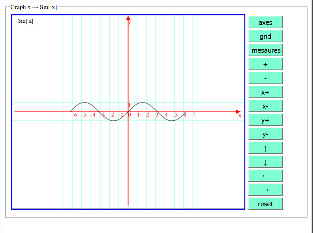
The rectangle containing the graph can be saved as an image in * .png format on a storage device of your system by clicking on it with the right mouse button. In the following examples we show only these images.
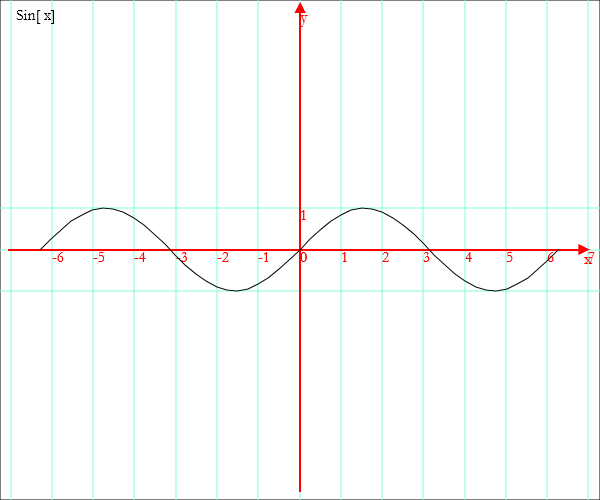
The buttons next to the rectangle containing the graph allow you to modify its appearance to improve its graphic rendering or to highlight some features.
For example, by clicking repeatedly on the button ![]() , the graph is enlarged.
, the graph is enlarged.
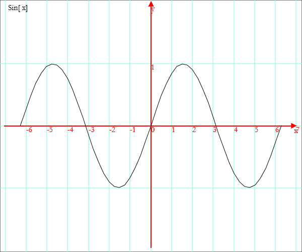
By repeatedly clicking the button ![]() , you increase the unit on the y axis.
, you increase the unit on the y axis.
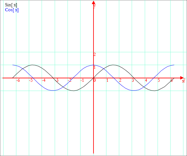
You can plot several functions together, inserting their names into a list delimited by braces.
Example.
Graph[x,{Sin[x],Cos[x]},-2P,2P]
You can get the graph of a previously declared function.
Example.
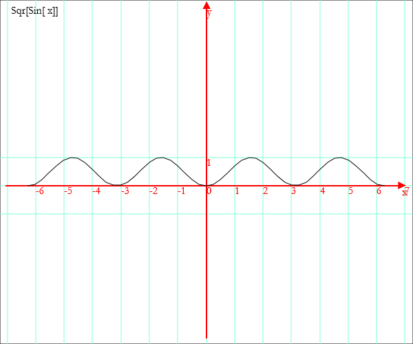
qsin[x]:=Sin[x]^2; Graph[x,qsin[x],-2P,2P]
or, more simply
Graph[x,Sqr[Sin[x]],-2P,2P]
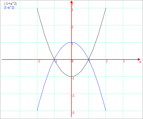
Also in this case you can plot several functions together.
Graph[x,{x^2-1,1-x^2},-2,2]
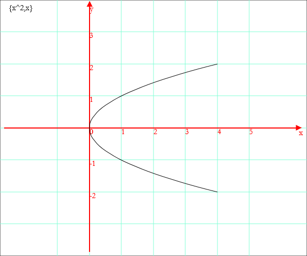
You can define a parametric function in the following way
f[x]:={x^2,x}
and obtain its graph
Graph[x,f[x],-2,2]
Geometric drawings
Simple geometric shapes are coded as lists of at least two pairs of coordinates. Once this list has been defined, the drawing is made with the operator Draw.
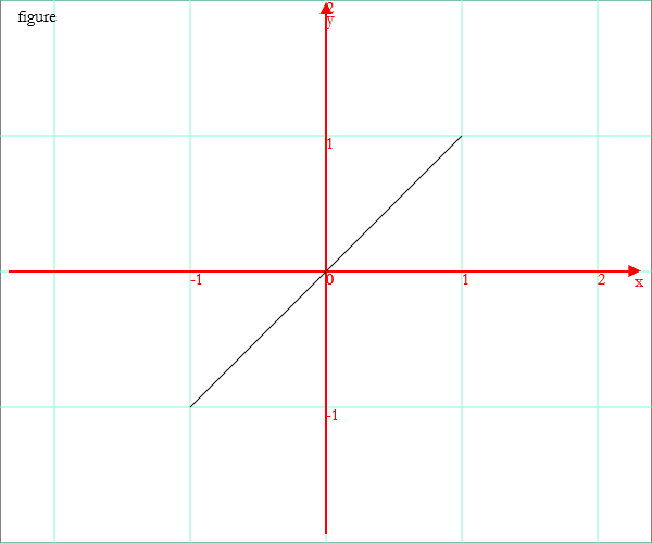
Example: a segment
Draw[{-1,-1},{1,1}]
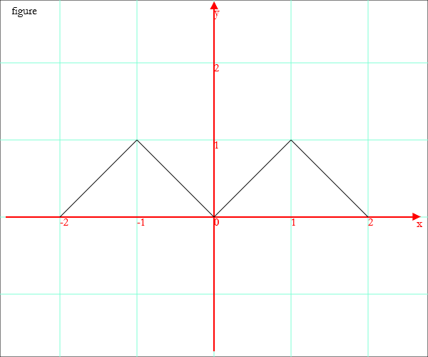
Example: a polygonal line
Draw[{-2,0},{-1,1},{0,0},{1,1},{2,0}]
You can represent regular polygons, circumferences, ellipses, arcs of curves defined by functions. To achieve these results, you must operate as follows:
generate the description of the drawing, assigning the output of one of the following operators to a constant identifier:
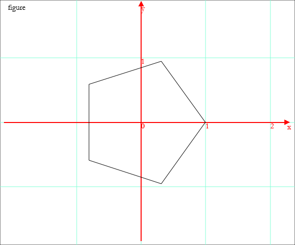
PoliVCircEllipseTranslateRotateDraw with argument given by one or more identifiers.Examples.
penta=PolyV[{0,0},1,5]; Draw[penta]
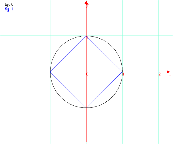
c=Circ[{0,0},1]; qu=PolyV[{0,0},1,4]; Draw[c,qu]
To represent arcs of curves described by functions, proceed as follows:
Produce a list of points with the operator Coords applied to the function identifier, to the defined interval and, if necessary, to the increment step
and assign the output of this operator to a constant;
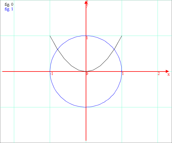
para=Coords[x,Sqr[x],-1,1,0.1]
Draw.Example
para=Coords[x,Sqr[x],-1,1,0.1]; c=Circ[{0,0},1]; Draw[para,c]
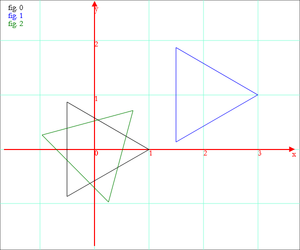
The description of a drawing can be translated or rotated; eg:
tri=PolyV[{0,0},1,3]; trasl=Translate[tri,{2,1}]; rot=Rotate[tri,45°]; Draw[tri,trasl,rot]
Histograms
You can represent two-dimensional histograms using the operator Histogram with argument given by list of pairs {number, number} or {string, number}.
The list must be preceded by a string with the title.
Example.
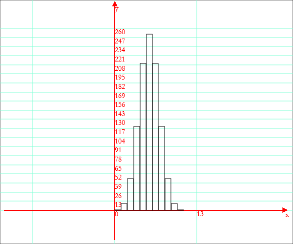
f[k] := Binomial[10,k]; Histogram["binomial coefficients",Coords[k,f[k],0,10,1]]
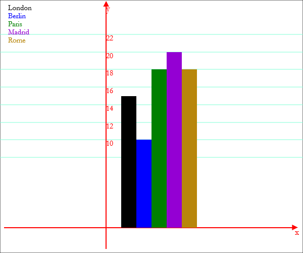
t = {"London",15},{"Berlin",10},{"Paris",18},{"Madrid",20},{"Rome",18}; Histogram["temperatures",t]
last revision: May 2018