The analysis of the properties of the gases, ie the aeriform substances at a high temperature and low pressure,
far from the physical conditions necessary for their liquefaction, led the physicists of the eighteenth century
and of the first decades of the nineteenth century to the following conclusions:
a given amount of gas with constant density and in condition of equilibrium, that is contained in a fixed volume
and with constant absolute temperature, exerts against the surfaces in contact with it forces directly proportional
to these surfaces (Pascal principle); the constant relationship between force and surface is called pressure.
equal volumes of gas, under the same conditions of temperature and pressure, contain the same number of molecules;
in particular a volume of 22,414 liters, at 0°C and with a pressure of one atmosphere (normal state), contains
about 6.023·1023 molecules; this quantity of gas is said mole and the number of molecules in one mole
is said the Avogadro's number, which will be hereinafter indicated with N;
in the isothermal expansions or compressions, volume and pressure are inversely proportional;
in the isochoric heating or cooling processes, the pressure is directly proportional to the absolute temperature.
in the isobaric heating or cooling processes, the volume is directly proportional to the absolute temperature.
The last three laws are collectively expressed by the equation of state of a gas, also known as the
Clapeyron equation, which, for one mole, is
where the proportionality constant R, the value of which depends on the units of measurement adopted for expressing volume V,
the pressure P and the absolute temperature T, is experimentally detectable by any thermodynamic state,
in particular from the normal state.
In S.I. units, R = 8.31 j/K·mole; if the volume is measured in liters and the pressure in atmospheres,
R = 8.21·10-2 l·atm/K·mole.
2. The work in the expansion of a gas.
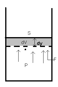
Let us suppose that has a gas has pressure P and is contained in a cylindrical vessel of section S and volume V.
Let us suppose also that the lateral surface of the cylinder and the base surface are rigid, while the upper surface is mobile.
The force F that the gas exerts against a surface of the container is proportional to the pressure and to the surface.
In particular, the force exerted against the movable surface is
If the force causes a raising dy of the moving surface, it does a work dW=Fdy.
that is, an expansion dV of the gas implies a positive work PdV.
This work, for the principle of conservation of mechanical energy, is produced at the expense of energy
of the gas, which decreases by an equal amount.
therefore
3. Temperature and energy in the ideal gas.
The need to reduce thermodynamics and mechanics to common principles led the physicists of the nineteenth century
to seek an explanation of the macroscopic properties of a gas in the dynamics of the molecules that constitute them.
A given amount of ideal gas is a system consisting of n point particles of equal mass m and distinguishable
each other. As they are punctiform, for each of them, at any instant, the position, the speed and therefore the kinetic energy
are classically determined. In addition we assume that the particles do not have mutual interactions, either with each other,
nor with the outside, and that therefore their potential energy is zero.
The system is confined in a container with rigid walls. The collisions of the particles against the walls are perfectly elastic.
Let us suppose, for simplicity, that the container is a cube of edge l, and choose as reference system a set of three edges
converging in the same vertex; then the speed of the i-th particle is described by the vector
If vix is different from 0, the i-th particle regularly collides against the walls Sx,
perpendicular to the x axis, with frequency
In each of these collisions vix changes sign, and therefore the absolute change of momentum at each collision is
In each time unit, each wall Sx receives from the particle a total impulse given by the product of the variation
of the impulse due to each individual collision multiplied by the number of collisions in a second, ie the frequency (3.1)
The impulse on the wall of all the n particles per unit time is given by the sum of all the ΔpSix
For the Newton's second law, the average force on the wall is given by the change of the impulse in the unit time
The mean pressure Px on the walls Sx is given by
Since l3 = V
In an analogous way, for the walls perpendicular to the other axes we obtain
By the Pascal's principle, Px=Py=Pz=P.
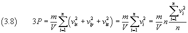
If we sum side by side the three previous equations, we get
If we represent the mean value of the squares of the speeds as
we obtain
If we consider one mole of gas, we have n=N, then from the equation (1.1) we get
The left hand side in the equation (3.11) is twice the mean kinetic energy of the molecules, so
With this equation we obtain a very important physical result: the macroscopic thermodynamical quantity absolute temperature
is the macroscopic manifestation of a mechanical microscopic quantity, that is, the mean kinetic energy of the molecules.
According to this equation, when the absolute temperature is equal to zero, all the molecules are at rest.
From the equation (3.12) we derive also the total energy
of an ideal gas consisting of n particles at absolute temperature T:
In particular, for one mole,
4. The first law of thermodynamics.
The mean kinetic energy of the particles is the mean value of the energies of the individual particles whose values,
in principle, can assume any positive real value: there may be particles at rest, slow particles, fast or fastest particles.
If we assume that the possible values of the energy of the particles are discrete and finite in number,
we can represent these values by εi;
in a given state of the system a number n1 of particles will have energy level ε1,
another number n2 of particles will have energy level ε2 and so on.
In general ni particles will have energy level εi.
We will say that the level of energy εi has the population ni.
If we represent by s the number of possible energy levels in a given state of the system, its total energy is given by
If we admit that the energy levels are so close, that we can think that the energy varies with continuity from one state to another,
and that the populations of the levels are so large, so that their variations can be considered infinitesimal,
assumptions acceptable when the number of particles is of the order of Avogadro's number, by differentiating the expression (4.1)
of , we obtain
The equation (4.2) shows that the variation of the total energy may occur by a combination of two processes:
due to the variation of the energy levels;
due to the variation of the population of the energy levels.
If we interpret macroscopically the two processes, we see that the first one
represents the variation in total energy attributable to the change of volume, ie the mechanical work;
the second one
represents the variation of total energy, not due to mechanical work,
lost or gained for the variation of the population of energy levels, ie the transfer of particles from one to another level of energy,
attributable to their acquisition or loss of energy in the absence of external work: the energy exchanged in this way is called heat,
and is usually represented by dQ.
In conclusion, the equation (4.2) can be written
The equation (4.3) is the macroscopic statement of the First Law of Thermodynamics.
5. The molar specific heats.
In an isochoric process, that is, with constant volume, a system does not make work, therefore, the first law of thermodynamics,
for one mole of monatomic ideal gas, is reduced to
then
The ratio in the left hand side is called molar specific heat and, since its value was obtained in a condition of
constant volume, the value obtained in this way is said molar specific heat at constant volume.
If we denote this quantity by cV we obtain
In an isobaric process, that is, with constant pressure, if we differentiate the equation (1.1), we obtain
Therefore the first law of thermodynamics, for one mole of monatomic ideal gas, becomes
then
The molar specific heat obtained in this way is called molar specific heat at constant pressure
and is denoted by cP:
The ratio of the two specific heats is usually written γ
The experimental measurements of γ for the real monatomic gas are in good agreement with that predicted by the
theory of the monatomic ideal gas. Instead, the measures on real gases with diatomic or polyatomic molecules give discordant values.
The problem can be overcome by assuming that the mean molecular kinetic energy is subdivided into equal portions, each one with value
for each degree of freedom of a molecule. Given that a monatomic molecule has only three translational degrees of freedom,
this hypothesis gives the value obtained in (3.12).
But for the diatomic molecules, for which we must consider five degrees of freedom, three of translation and two of rotation,
the mean molecular kinetic energy must be
6. The Poisson's equation for the adiabatic processes.
The changes of the state of a system that occur without heat exchanges with the outside are called adiabatic processes.
In an adiabatic process, for one mole of a monatomic ideal gas, the first law of thermodynamics is reduced to
Differentiating the equation (1.1), we obtain
From (6.1) and (6.2) we get
We see that 5/3 is the value of γ; if we divide both the sides by PV and integrate, we get
The equation (6.7) expresses the Poisson's law for the adiabatic processes.
7. The evolution of an ideal gas.
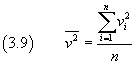
Let us suppose that a system is formed by 5 particles, each of which may have energy εi
equal to 1, 2 or 3 arbitrary units with respective probabilities p1=0.3, p2=0.5, p3=0.2.
The possible configurations of the system are described in the following table.
The knowledge of the total energy of the system, for example 10, in general is not sufficient to uniquely identify the status
of the system, because this value of the total energy can be produced by different states of the system itself, that is,
S9, S12 and S16.
The principle of conservation of energy does not prevent the transition of the system from one state to another of equal energy.
But these the states have different probabilities.
Since the particles are distinguishable, the probability
of a state is obtained by multiplying the probabilities that the particles have a given energy by the number of the
possible permutations of the particles between them.
For example, the probability of the state S9 is given by the product
multiplied by the number of possible different permutations of the sequence aabcc, which are
Therefore, for the state S9, we obtain the probability shown in the table
With the same method we obtain the probabilities of other states. In particular the state S12 has probability 0.15
and the state S16 has probability 0.031. We note that the state S12, for the same energy, has much higher probability
than the other two states.
It will be reasonable to expect that the most stable configuration of the system is that which corresponds
to the maximum probability..
When the number of particles is of the order of Avogadro's number, the maximum probability is so great, compared with
the probabilities of the other isoenergetic configurations, to ensure that the state which corresponds to this maximum is so stable that,
if the system is in this state, the transition to other states of equal energy is impossible.
We can therefore state the following principle: the configuration of thermodynamic equilibrium of a system of n particles
and with given total energy coincides with its most probable configuration; the system evolves spontaneously towards
such configuration and when it is reached it is impossible that the system returns spontaneously to other configurations.
Generalizing the method used to calculate the probability of the state S9 of the proposed example, we conclude that the probability P
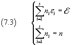
that n particles are distributed in s states ε1, ε2,...εs with
respective probabilities p1,p2,...ps and populations n1,n2,...ns is
We denote the multipliers by α e β and construct the function F(n1,n2,..ns)
The maximum of ln P is obtained by imposing that the total differential of F is zero, that is, by solving the system
then
with the conditions (7.3).
From the equation (8.9) we get
and, with obvious substitution,
This equation expresses the population ni of the state of energy εi as a function of the
the energy εi itself and the probability pi that a particle has such energy,
and is said Boltzmann distribution.
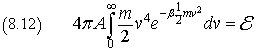
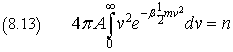
If we assume that the energy is the kinetic energy
In classical mechanics, the kinetic energy varies continuously as a function of the continuous variable v,
so n is also a continuous function of v. n(v) represents the number of particles having speed v,
the probability p is proportional to the number of particles that have the square of the speed between
v2 and (v+dv)2. This number can be geometrically represented as a spherical shell with radius v
and thickness dv and its size is 4πv2dv.
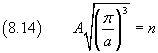
If the variables are continuous, the sums in (7.3) should be replaced by integrals
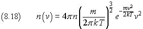
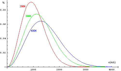
The function (8.18) shows that the population of the low energy states and that of those of high energy tends to zero
and that the maximum value of n(v) increases with temperature.
Example: percent distrubution of the speeds of the molecules of Helium at 200K, 300K, 400K.
9. Entropy.
As we saw in the previous section, the state with highest probability is derived from the condition that the differential of F,
described in (8.7), is equal to 0. This implies
If the system is in equilibrium, each ni is constant, then d(ln P) = 0.
But if the system, while the number of particles and the total energy and thus the temperature remain unchanged,
may redistribute the particles among the various energy levels, the differentials dni will not be all zero.
However their sum will be always equal to 0. In this case
The sum which appears in the right side of the equation (9.2) is the same that appears in (4.2)
and which has been macroscopically interpreted as the heat exchanged by the system. Then
Using the expression of β obtained in equation (8.16) we get
Denoting by dS the ratio between dQ and T, we have
and then
The quantity S, called entropy, is a macroscopic quantity, as it is defined in terms of the macroscopic quantities Q and T.
We observe that the equation (9.5) defines only the differential of this quantity, then its variation, not its absolute value and,
consequently, in the equation (9.6), S is expressed up to an additive constant.
The entropy is directly proportional to the logarithm of the probability of the microscopic configuration of the particle system
and then, if we assume that a system evolves spontaneously towards the configuration of maximum probability,
it follows that an ideal gas spontaneously evolves toward a state of maximum entropy.
This statement is known as the Second Law of Thermodynamics.